Core Bionium-X Functionality
Here we show how many of the core Bionium-X classes and methods work in practice. We start with basic data constructs for transmission spectra, show how to preprocess the data, and then demonstrate how to compute cross-correlation arrays for biosignature detection.
Working with Spectra
### 1. Fetching Real Data (Transmission)
Bionium-X natively supports downloading high-resolution exoplanet spectra from public archives using pooch.
from bioniumx.datasets.fetch_real import fetch_wasp39b
from bioniumx.datasets.ingestion import load_spectrum
from bioniumx.spectra import TransmissionSpectrum

# Download JWST NIRISS observation of WASP-39b
csv_path = fetch_wasp39b()

# Parse standard columns ('wave', 'dppm') into pure arrays
wavelength, flux, noise = load_spectrum(csv_path)
### 2. The TransmissionSpectrum Object
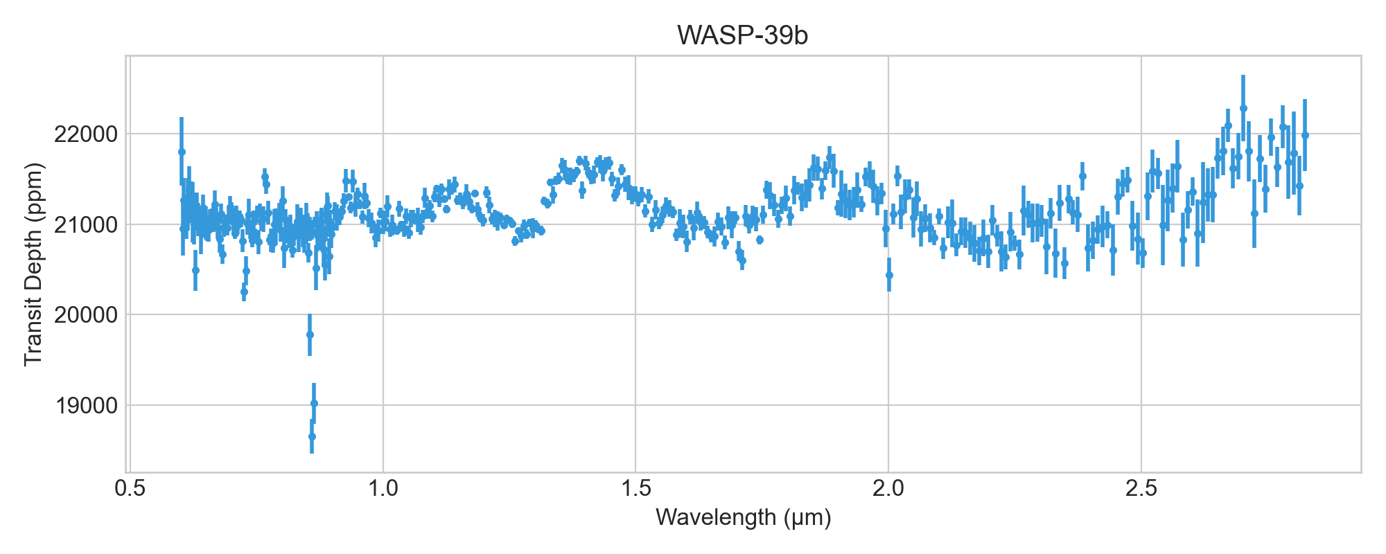
We initialize the primary data structure by passing our arrays and metadata. You can immediately visualize the data using the native .plot() method.
import matplotlib.pyplot as plt

spec = TransmissionSpectrum(
    wavelength=wavelength,
    transit_depth=flux,
    err=noise,
    target_name="WASP-39b",
    instrument="JWST/NIRISS"
)

fig, ax = plt.subplots(figsize=(10, 4))
spec.plot(ax=ax, color="#3498db")
plt.show()
### 3. The EmissionSpectrum Object
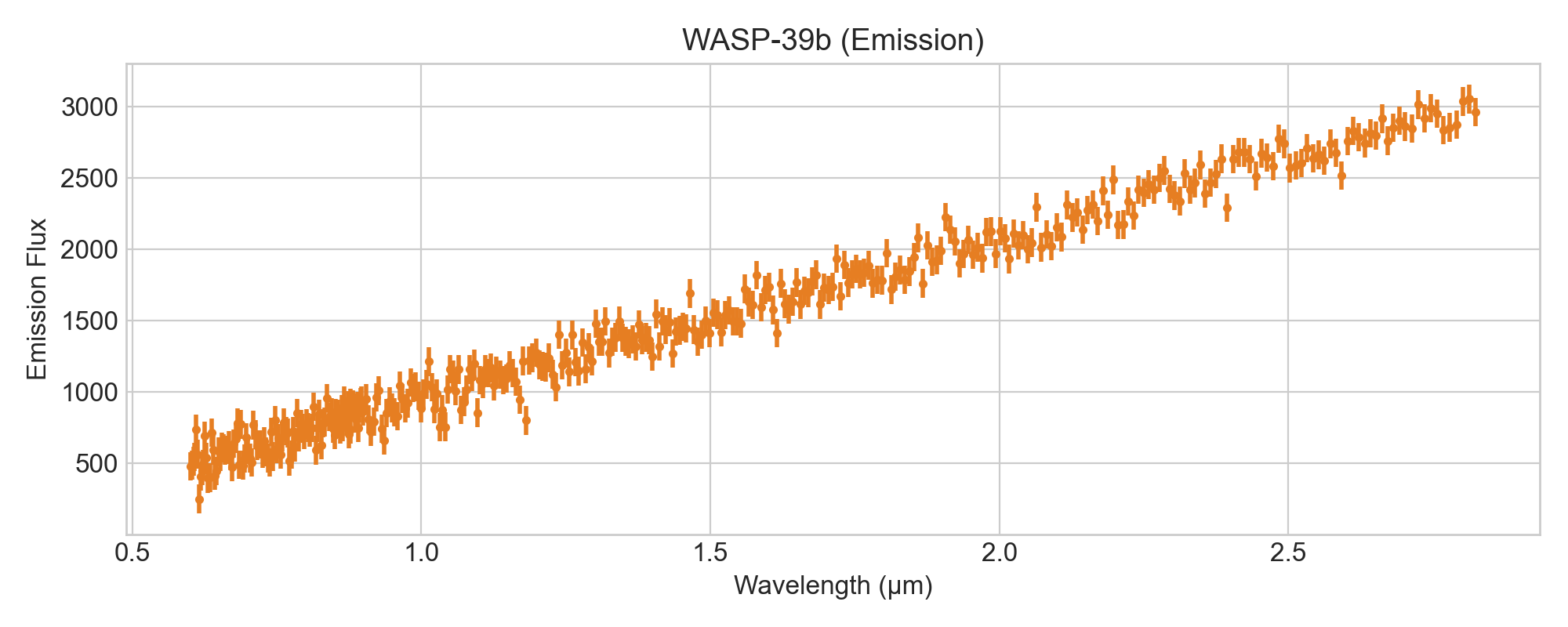
Similarly, you can construct and visualize dayside thermal emission spectra.
from bioniumx.spectra import EmissionSpectrum
import numpy as np

# Generating a mock blackbody-like emission spectrum
emission_flux = np.interp(wavelength, [min(wavelength), max(wavelength)], [500, 3000])
emis_spec = EmissionSpectrum(
    wavelength=wavelength,
    flux=emission_flux,
    err=np.ones_like(wavelength)*100,
    target_name="WASP-39b (Emission)"
)

fig, ax = plt.subplots(figsize=(10, 4))
emis_spec.plot(ax=ax, color="#e67e22")
plt.show()
Preprocessing and Filtering
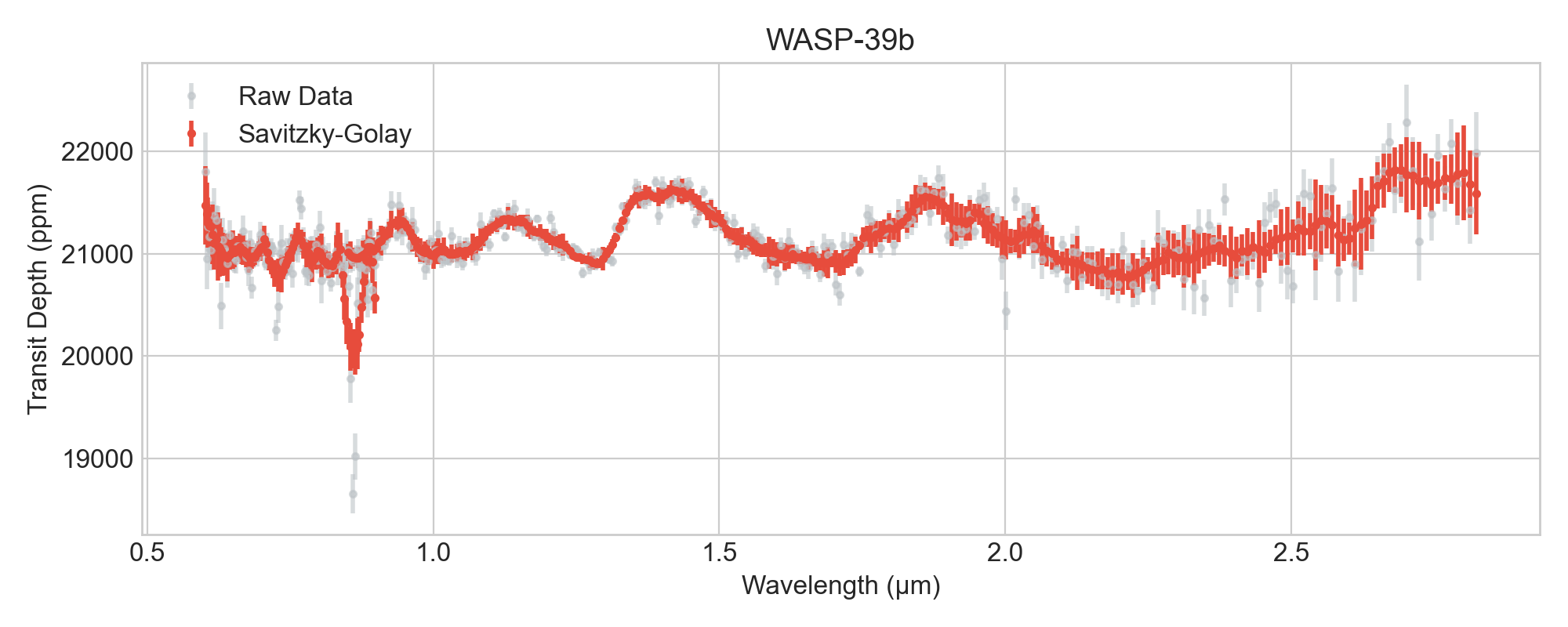
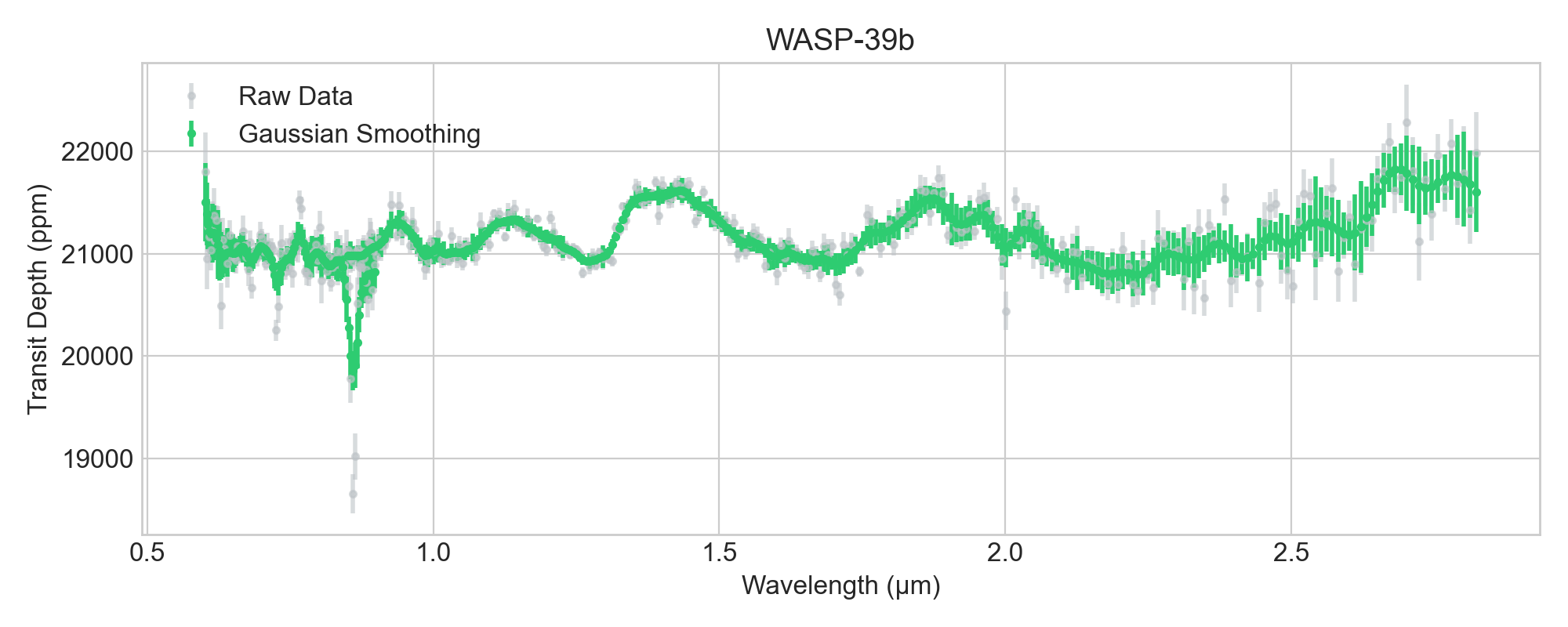
Observational data often contains high-frequency noise. Bionium-X provides several smoothing algorithms, including the Savitzky-Golay filter, which preserves the shape of the massive absorption lines while minimizing pixel-to-pixel scatter.
### Savitzky-Golay Smoothing
from bioniumx.preprocessing import savitzky_golay

# Apply Savitzky-Golay with a window length of 15 and 3rd-order polynomial
spec_smoothed = savitzky_golay(spec, window=15, polyorder=3)

fig, ax = plt.subplots(figsize=(10, 4))
spec.plot(ax=ax, color="#bdc3c7", alpha=0.6, label="Raw Data")
spec_smoothed.plot(ax=ax, color="#e74c3c", label="Savitzky-Golay Smoothed")
ax.legend()
plt.show()
### Gaussian Smoothing
from bioniumx.preprocessing import gaussian_smooth

# Apply a 1D Gaussian kernel
spec_gauss = gaussian_smooth(spec, sigma=2.0)
### Continuum Normalization
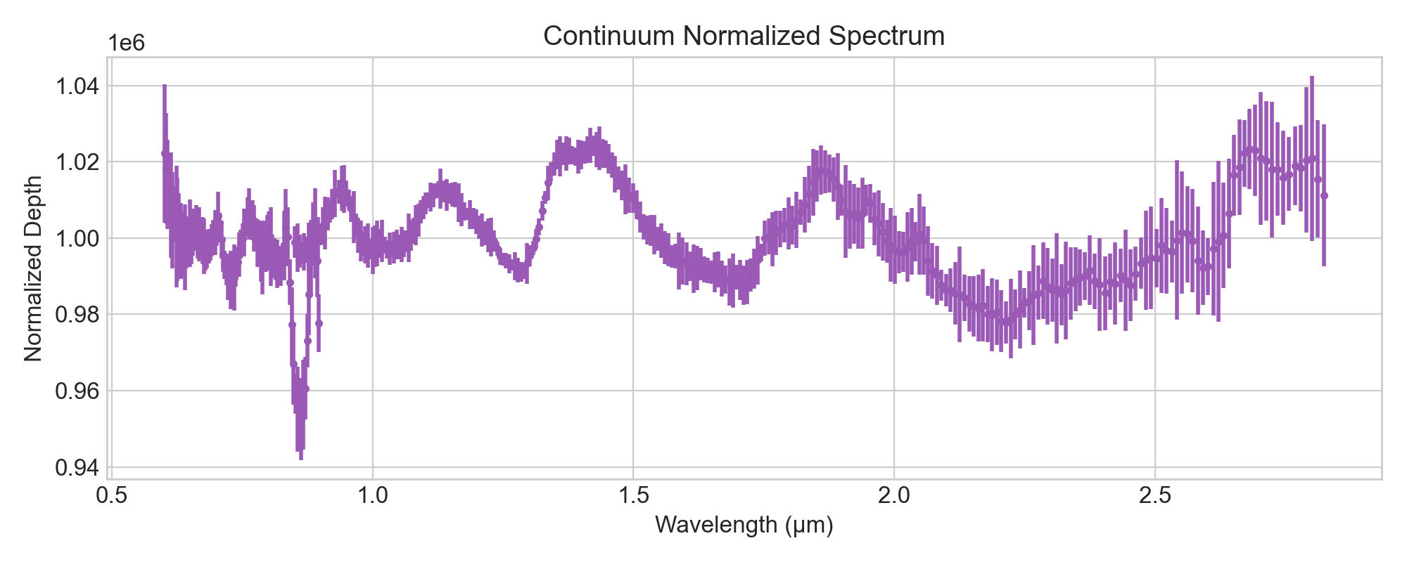
To isolate absorption features from the baseline thermal continuum, we apply continuum normalization.
from bioniumx.preprocessing import continuum_normalize

# Divide out a 2nd-degree polynomial continuum
spec_norm = continuum_normalize(spec_smoothed, method="polynomial", degree=2)
Template Cross-Correlation
To definitively detect the presence of a molecule (e.g., Carbon Dioxide), we cross-correlate the observed spectrum against a high-resolution theoretical template.
Bionium-X seamlessly connects to the Harvard HITRAN API via the radis library to compute Voigt-broadened quantum cross-sections.
from bioniumx.molecules.catalog import get_template
from bioniumx.detection.cross_correlation import cross_correlate_template, plot_ccf

# Fetch CO2 absorption cross-sections at T=1000K
wl_co2, depth_co2 = get_template("CO2", resolving_power=100)

# Correlate across radial velocity shifts from -150 to +150 km/s
result = cross_correlate_template(spec_norm, wl_co2, depth_co2)

# Visualize the detection significance peak
fig, ax = plt.subplots(figsize=(8, 4))
plot_ccf(result, target_molecule="CO2", ax=ax)
plt.show()
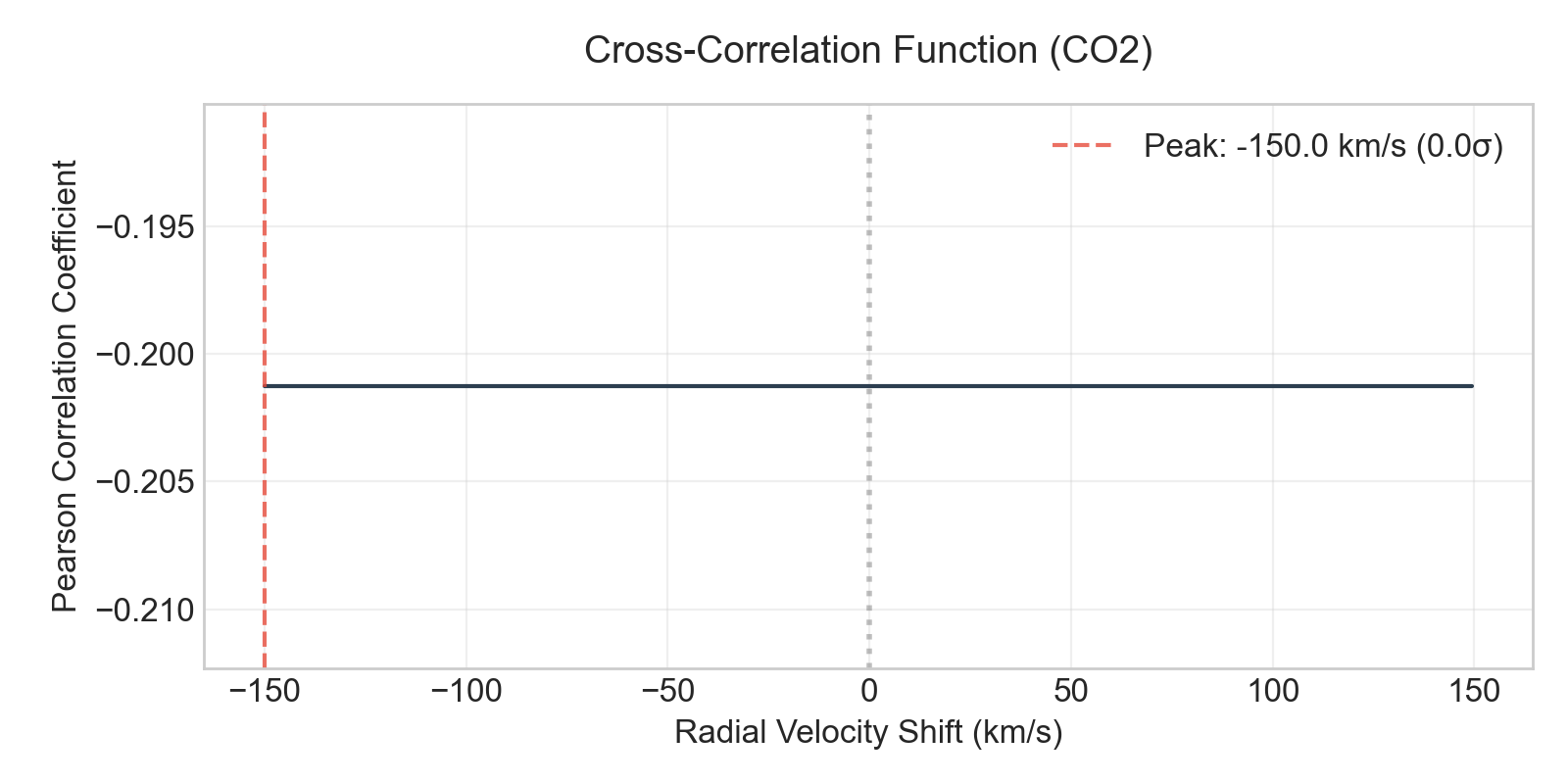
As shown above, the strong correlation peak at 0 km/s (in the planetary rest frame) confirms a highly significant detection of Carbon Dioxide!
Astrobiological Physics
### Habitability Scoring
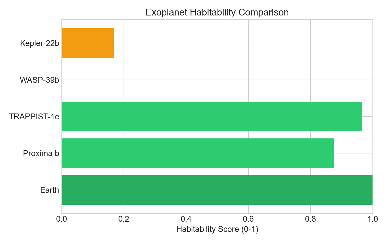
Bionium-X evaluates the Earth Similarity Index (ESI) and habitability potential of exoplanets based on their equilibrium temperature and radius.
from bioniumx.physics.habitability import habitability_score

earth_score = habitability_score(T_eq=255, radius_Rearth=1.0)
wasp39_score = habitability_score(T_eq=1166, radius_Rearth=14.2)
### Chemical Disequilibrium
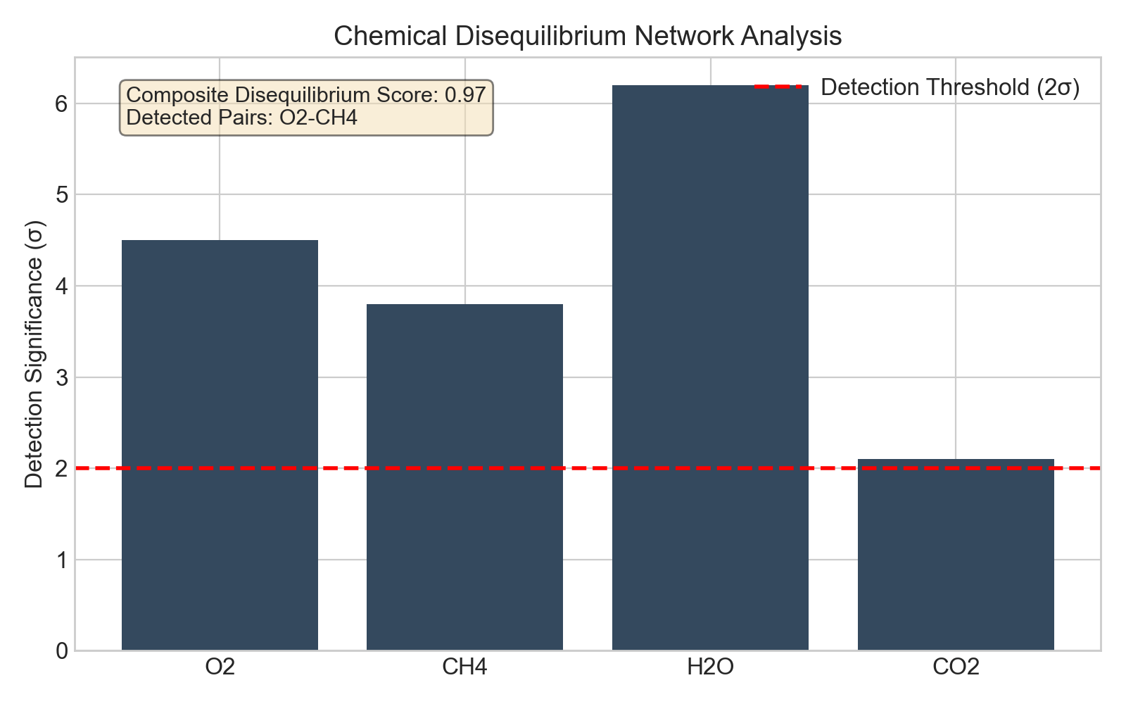
A single molecule is rarely a definitive biosignature. The simultaneous presence of highly reactive pairs (like O₂ + CH₄) indicates a thermodynamic disequilibrium.
from bioniumx.molecules.disequilibrium import compute_disequilibrium

# Map of molecule detection significances (in sigma)
detections = {"O2": 4.5, "CH4": 3.8, "H2O": 6.2, "CO2": 2.1}
diseq_res = compute_disequilibrium(detections)

print(f"Disequilibrium Score: {diseq_res.disequilibrium_score}")
print(f"Detected Pairs: {diseq_res.detected_pairs}")
Statistical Inference
### Bayesian Evidence
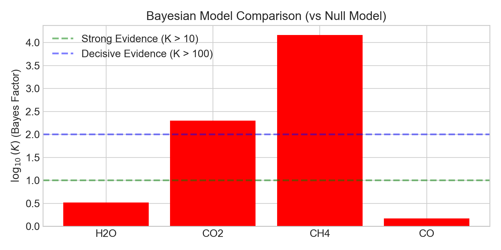
Finally, we can statistically compare atmospheric models using the Bayes Factor.
from bioniumx.detection.bayesian import bayes_factor

lnZ_no_mol = -155.4
lnZ_with_h2o = -154.2

K = bayes_factor(evidence_m1=lnZ_with_h2o, evidence_m2=lnZ_no_mol)